Tag Archives: Network

Availability Requirements Engineering Video

[008] Using a System Model for Iterative Availability Management

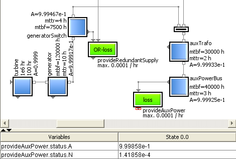
Using a System Model For Iterative Availability Management, Power Supply System ExampleThe description of the last post [007] showed, how we added related quantities and arithmetics to compute availability and non-availability for individual items. This extension made them smarter and also added some “decoration” to display the parameter values.

Today’s video post guides us from item level back up to system level. At the end of the day, it is the availability of a system – or better: of certain system functions – that we are interested in.


Simply by using the amended versions of the original item classes allowed it to extend the benefit of the existing system model – here in the example of the power supply system – without actually having to touch and modify it in any way. The topology remains the same as already known and graphically specified before.

The idea is, that the individual topological context of an individual item not only determines its functionality, but also the computation of the availability of a service that this item shall provide. That means, not only its own “standalone” properties of the relevant parameters – like MTBF and MTTR as shown in post [007] – determine the service availability, but also its individual supplies have to be taken into account.

According to the local dependencies of the individual item the behavior description of its unique category automatically provides the correct arithmetics to compute this availability value. That makes it very easy to compute the availability of a system, since the computation equation is assembled automatically, just by graphically connecting the various outputs and inputs of the used items – independent if they represent real hardware components, process steps or e.g. logistical activities.

Having direct and interactive access to all relevant parameters allows to easily modify values of Mean Time Between Failures MTBF or Mean Time To Repair MTTR of any item. Just by doing a system simulation it immediately becomes clear, if these modifications help to come closer to the target number – like five nines – or also the MTBF or MTTR requirements of other items have to be tightened.

So using a graphical hierarchical system model to iteratively find out optimal target values for the items or item categories – including the feature to save and load scenarios – adds a great flexibility to the process of availability management or specification. In a later post we plan to support this process even more by considering also criteria like cost or time to get a better idea of the performance of designated assembly architectures.

In this example we assumed that the parameters MTBF and MTTR – as some of the main drivers of item availability – were given. But they are just some statistical values and depend on other properties as well. How the target function availability of a system really is affected in case a certain item is down, will probably be the topic of post [009].

For the time being, feel free to get in contact with us. Get in contact ...

Reliability Standards

[003] Reliability Modeling from Fault to Failure

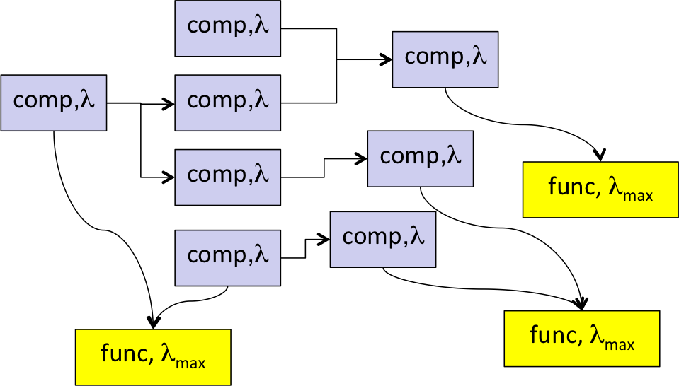
Components And Functions In System Design, Determining the reliability of systemsOne of the core features to investigate in the context of RAMS analyses is the functional reliability of the system. Quantitatively represented by the failure rate lambda, it specifies the number of failures within a certain time period, e.g. “failures per million hours (fpmh)”.

Again as in post [001] we clearly have to distinguish between failure rates of system functions and of system components, as shown in the figure.


At the start of the design process what is given are probably upper limits of the failure rates of the functions – not the components (!) – of the designated system. These individual maximal values for lambda might be defined by the customer, by specification, by design rules, by standards (i.e. IEC 61508, ISO 26262, MIL882D etc) or otherwise. When developping a flexible block-library we need to represent this given parameter lambda_max by a value slot on function level.

On the other hand what has to be determined is each functions actual failure rate, say lambda_act. It depends mainly on 2 factors:

  1. the failure rate lambda of each directly or indirectly required component, i.e. its quality
  2. the system topology, how the components are connected and interact, i.e. the design architecture.

Concerning components quality, we simply provide a value slot on component level to represent the individual lambda. In the easiest case it will be just a fixed parameter for lambda. More ambitious approaches, like dependencies of the component’s failure rate on other environmental usage parameters, can be considered. In industrial practice also the “mean time between failures (mtbf)” is frequently used, which – under common conditions – is the inverse of the failure rate lambda.

Concerning system topology,. we need an arithmetic to consider the topology when determining the actual function failure rates. This is basically not too complicated, if we look at the system on a smaller, local or component scale instead trying to derive the calculation on global level. Assuming independence of the suppliers of a component, it follows simple rules, very similar to those applied in classical Fault Tree Analysis FTA:

  1. Add up the probabilities of the individual failures, if each of them separately might “kill” the output. Example: The probability that an individual component fails to deliver its output service, is the sum of its own failure rate and the probability that its immediate supply fails.
  2. Multiply the probabilities of the individual failures, if only the combination will “kill” the output. Example: The probability that the redundant supply of a component fails, is the product of the failure rates of the individual supplies.

Applying these rules recursively from the function viewpoint dependent on the individual redundancy situation at each component and its inputs, up to the first elements in the supplier-consumer-path, is a major step to modularize the failure rate computation of each function.

How closely related Fault Tree Analysis FTA and Root Cause Analysis are will be shown in post [004].

Architecture Product Development Safety Video

[002] The safety viewpoint – from faults to failure

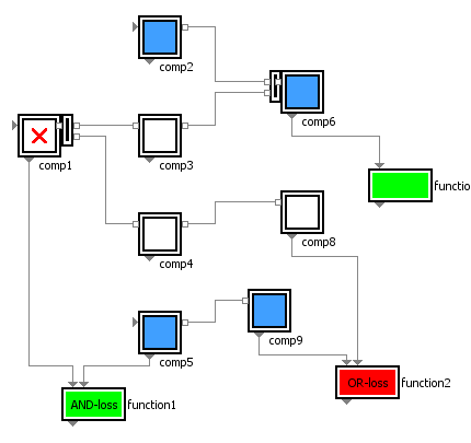
Schematics components fault leading to function failureIs functionality all we need? Are we done when we have found an architecture by which all functions work? – Yes and No!

Under the aspect of safety we also have to consider the inverse view and ask, under which conditions which function will fail. If an individual component fails, it might affect the various system functions in different ways. Redundancy plays a crucial role here.

When does a function fail? [more…]Dependent on its internal requirements, it will fail if one or several of its supplying components fail. The one at the end of the functional path. And this one will fail, …

  • … if itself is defective or
  • … if one or several of its own suppliers fail.

Recursively we can track back the whole functional network, a network of suppliers and consumers of services. Each with an individual internal condition. In the simplest form this may be expressed by simple logic, Boolean logic.

The following video shows some failure cases of the system in the figure shown in post [001].. Square boxes represent the components, rectangular ones the functions.

The blocks used here incorporate basically not more than such generic Boolean conditions. If a component provides an expected output – like “energized” – it is displayed in blue. If it provides no signal, it is white. And a nominally working function is green, while a failed function shows up in red. The analysis might remind you to FMEA – we’ll come back to that later.

The clue is, that each component may interactively set to “fails”, which means it fails to deliver its own service, locally, independent of its incoming supply. As the video shows, a simple simulation of such a network will immediately unveil, which functions will be affected by which component faults – indivudual ones or also combinations.

After having clarified these basic dependencies, we will introduce the concept of failure rates in post [003].