Category Archives: Reliability

functional reliability, component reliability, reliability analysis, lambda, mtbf

Availability Reliability Requirements Engineering

[007] Amending Item Models by MTTR and Availability Computation

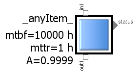
Item model with parameters MTBF and MTTR and associated item Availability, displyed as simple block iconIn this post we’re going to amend the existing library blocks by the quantities and arithmetics introduced in post [006] and see how this can facilitate the computation of the availability of a system.

What we need in the first step are the required variable and parameter slots, assigned to each individual item. For the time being we assume that the Mean Time To Repair MTTR is given as a known parameter for each item with the default unit of hours.


In the Modelica modeling language, parameters are quantities whose value has to be assigned prior to a simulation run, i.e. they will not be calculated. In that aspect the parameter type differs from normal variables. We plan to consider also other ways to determine and represent the MTTR and will describe this in future posts.

Cartoon, Maintenance and Lubrication, Improving Mean Time Between Failures MTBFSince the Mean Time Between Failures MTBF has been introduced in a similar parametric way in the default item, the local availability A of this particular item may immediately be calculated according to the arithmetics in post [006]. So if the pre-assigned parameter values of MTBF is 10000 hours and the Mean Time To Repair is 1 hour, this results in a local item availability of 0.9999 or 99.99%. In case we want to achiev 99.999% i.e. five nines, we would have to modify e.g. MTTR to 0.1 hour – i.e. speed up the repair action – or increase MTBF to 100000 hours – i.e. get higher-quality parts. Since such modifications can be done interactively “on the fly”, this might help the system engineer to specify the quality requirements.

We may specify in the item graphics, that these parameter values shall be displayed besides the visual icon, along with the individual name (see intro figure).

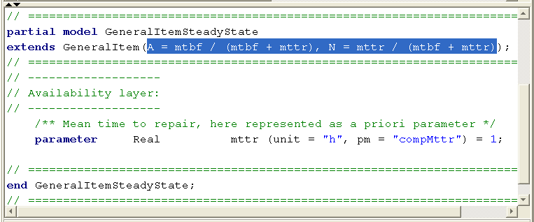
As the modeling approach follows an object-oriented concept, all item models are derived from one general item class and we need to do these declarations only at a single spot in the library. The next figure shows how this new functionality can be implemented very quickly in a few lines of code in the internal modeling language. Its only a reference to the GeneralItem master model, the equations for A and N and the declaration of the mttr parameter in a one-liner:

Amending the base class by parameters and arithmetics to compute the Availability and Non-Availability of an item

Before we proceed, it’s important to understand what we really have achieved now. We have just added the parameter MTTR to the master item description in the library. Such an item might represent various things like

  • a certain technical hardware unit within a machine,
  • a process step within a bigger procedure,
  • an adminstrative item within an organisation
  • or any other kind of element in a bigger context.

Together with the already existing parameter MTBF this allowed us to compute the also newly introduced availability quantity A. However, this item availability value is rather a theoretical value, describing a statistical value of this “box” in a standalone view, assuming that it is properly supplied.

In a real system, such an item almost never exists isolated. Instead, it will be connected to and interacting with its neighbors in a more or less complex environment. So in order to compute the actual service availability at the output of this box, we have to consider also the individual supply situation at its input. This will be the topic of post [008], then allowing us to efficiently compute the service availability of the power supply system from post [005]. And the good message is: this is possible without having to touch the overall system model!

Thanks for sharing this article!

Availability RAMS Reliability

[006] Computing the Availability of a System, some Basics

Cartoon Maintenance, Computing the Availability of a system, five ninesSimilar to the concept of Reliability computation introduced in post [003], we also would like to support the computation of system Availability with the model blocks. However, before talking about the availability arithmetics, again we have to clarify its meaning.

So what is system availability? – Basically, a system can be “up” and operating, i.e. providing the required service, or “down” and non-operating, i.e. not providing the service. Being in downtime can be planned (e.g. scheduled maintenance) or unplanned (e.g. irregular failure of system parts). Dependent on the required work effort, the need and delivery time of spare parts, the qualification of the repair and maintenance team etc. it takes more or less time to repair the system and get it back into the desired “Up”-mode.


While Reliability is used to express, how probable it is that a certain desired functionality of a system fails within a given period of time, the feature of Availability quantifies the operating time within such a period. Simply put, Wikipedia summarizes Availability being “the proportion of time a system is in a functioning condition”. (If interested, please look up more explanations there.)

Besides the already mentioned MTBF, important additional calculation symbols in this context are:

  • A: the symbol denoting the Availability of the respective part, item or service with theoretical values between 0 and 1, but practically usually being close to one, e.g. in high availability systems the magic “five nines” like 0.99999 or in percent this value is 99.999%, meaning 5 minutes per year (!);
  • N: the symbol denoting the Non-Availability of the respective part, item or service and the complement to A, i.e. the sum of A and N is always 1;
  • MTTR: the symbol denoting the Mean Time To Repair, the time needed to repair the system and get it back to service. To be correct, this time is not only needed for repair, but often is used to represent the complete downtime period, including fault detection and reporting, parts ordering (and delays), assembling, testing, start-up etc.

With these variables and stochastical parameters, the basic equations to compute the availability of a system item is:

A = MTBF / (MTBF + MTTR).

Although this maybe looks like a quite familiar equation, it is important to have a clear picture, to what these quantities really relate. Ok, MTBF and MTTR are kind of statistical parameters that have been estimated or gathered from the field and clearly can be associated to individual components. But with respect to A, we referred to certain services or functions of an item, that shall be available.

As long as we talk about system items providing only one single service, this distinction between components and their provided functions might appear artificial and not be so obvious: we can clearly observe it being Up or Down and there is a 1:1-mapping between the hardware and the functionality.

But as soon as we consider hierarchical systems or sub-systems that provide more than one single service or function, it is important to have proper and separated variable slots for the availability of system components and system functions, according to the orthogonal view we introduced earlier.

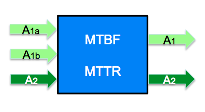
In terms of building-blocks of the SmartRAMDependencies of component output availability on inputs, MTBF and MTTRS-library in the “Availability layer” we need to provide MTBF and MTTR parameter slots only once for each component. However, concerning availability, variable slots have to be provided for each interacting service, the outgoing and the incoming ones, as illustrated in the picture. Thanks to the modular port-concept of Modelica, extending the already existing interfaces – or ports – by an additional variable for A is a matter of just one single model statement.
This were some basic thoughts about the required variable slots. Adding also the required arithmetics to the existing model classes and demonstrating it along the emergency power system that we used in the risk assessment example will be topic of post [007] .
 

Architecture RAMS Reliability Requirements Engineering Safety Video

[005] Risk Assessment Example: An Emergency Power System

Potential hazard in case of Aux power failure in a nuclear power station, Fukushima I by Digital Globe BIn the last posts we emphasized the basic system engineering concept of a clear distinction between

  • system components – or items in the wider sense – and
  • system functions.

Today’s video post shows a way to support this concept by modular RAMS blocks in a basic risk assessment example: the analysis of an emergency power system. An auxiliary power bus has to provide the electricity used for internal operations in a nuclear power station, like cooling pumps, control system or manipulating the nuclear fuel elements. So power failure on this Aux bus is surely a safety-critical event or hazard.


Using a modular, graphical system model allows to easily evaluate the effects of a local component failure – which might remind you to the common FMEA procedure – and automatically determine all possible root causes of a system function failure. But the  risk assessment procedure is supported also quantitatively, by assigning

  • by assigning individual MTBF values and failure rates on component level and
  • defining an upper limit of the “to-be”-failure rate on function level.

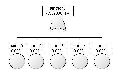
The fault tree for each undesired event of a failed function – the hazard in this risk assessment example – is derived automatically. So we can easily check if the failure rate requirements are met by anticipated architectural design of the power supply system and the quality of the component.

Although this system is comparatively simple and has two fully separated and independent branches, the example shows the benefit of the option to quickly change parameters of components or functions and to – in a wider scope – support also the requirements engineering process. In a later contribution we will analyze also seemingly independent supply branches, but which have hidden dependencies in form of common components or even common cause of failure. (Please note that the selected failure rate values just serve as placeholders here.)


In post [006] we will introduce the idea of availability modeling and the appropriate layer in the SmartRAMS library that allows to quickly determine the availability of a system.


Architecture Product Development RAMS Reliability Safety Video

[004] From Root Cause Investigation to Fault Tree Analysis

Example Fault Tree Analysis FTA, generated automatically from a component modelIn post [003] we referred to “each directly or indirectly required componen“, when talking about determination of the system function’s failure rate. But which components are required? – Well, basically all these individual items or combinations of items whose local failure will affect the considered function in a way that it does not work any longer.


In other words, we have to find out those components that are crucial for the functionality. A common way of doing that is a so-called root-cause investigation, assuming the individual function has failed.

One aspect of this post’s video is the demonstration, how these root-causes can easily be derived from the functional system model, using a kind of automatic backward reasoning. For each detected root-cause – be it a single fault, double fault or even higher order fault – the graphic of the connected SmartRAMS-blocks displays the affected system parts for each particular scenario.

Root cause analysis is often performed during system operation – i.e. late in the product life cycle – during diagnosis or troubleshooting. However, its reasoning and findings are very related to the top-down investigation in the context of a Fault Tree Analysis FTA, usually performed very early in product development.

Risk analysis by FTA has the goal to check if the safety and reliability requirements are met by the anticipated architecture. The system model composed from the simple Boolean library items supports also this purpose. We can automatically derive the Fault Trees and – as a side effect – compute the function failure rates from the component’s lambda-values. This is the other aspect shown in the video:


In post [005] we are going to demonstrate these features using a emergency power system as a simple risk assessment example.


Reliability Standards

[003] Reliability Modeling from Fault to Failure

Components And Functions In System Design, Determining the reliability of systemsOne of the core features to investigate in the context of RAMS analyses is the functional reliability of the system. Quantitatively represented by the failure rate lambda, it specifies the number of failures within a certain time period, e.g. “failures per million hours (fpmh)”.

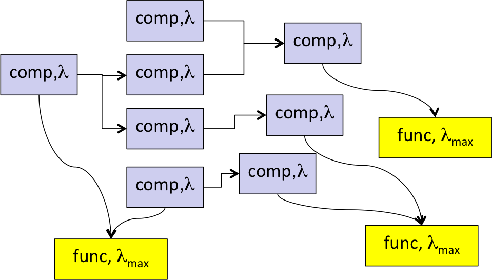
Again as in post [001] we clearly have to distinguish between failure rates of system functions and of system components, as shown in the figure.


At the start of the design process what is given are probably upper limits of the failure rates of the functions – not the components (!) – of the designated system. These individual maximal values for lambda might be defined by the customer, by specification, by design rules, by standards (i.e. IEC 61508, ISO 26262, MIL882D etc) or otherwise. When developping a flexible block-library we need to represent this given parameter lambda_max by a value slot on function level.

On the other hand what has to be determined is each functions actual failure rate, say lambda_act. It depends mainly on 2 factors:

  1. the failure rate lambda of each directly or indirectly required component, i.e. its quality
  2. the system topology, how the components are connected and interact, i.e. the design architecture.

Concerning components quality, we simply provide a value slot on component level to represent the individual lambda. In the easiest case it will be just a fixed parameter for lambda. More ambitious approaches, like dependencies of the component’s failure rate on other environmental usage parameters, can be considered. In industrial practice also the “mean time between failures (mtbf)” is frequently used, which – under common conditions – is the inverse of the failure rate lambda.

Concerning system topology,. we need an arithmetic to consider the topology when determining the actual function failure rates. This is basically not too complicated, if we look at the system on a smaller, local or component scale instead trying to derive the calculation on global level. Assuming independence of the suppliers of a component, it follows simple rules, very similar to those applied in classical Fault Tree Analysis FTA:

  1. Add up the probabilities of the individual failures, if each of them separately might “kill” the output. Example: The probability that an individual component fails to deliver its output service, is the sum of its own failure rate and the probability that its immediate supply fails.
  2. Multiply the probabilities of the individual failures, if only the combination will “kill” the output. Example: The probability that the redundant supply of a component fails, is the product of the failure rates of the individual supplies.

Applying these rules recursively from the function viewpoint dependent on the individual redundancy situation at each component and its inputs, up to the first elements in the supplier-consumer-path, is a major step to modularize the failure rate computation of each function.

How closely related Fault Tree Analysis FTA and Root Cause Analysis are will be shown in post [004].