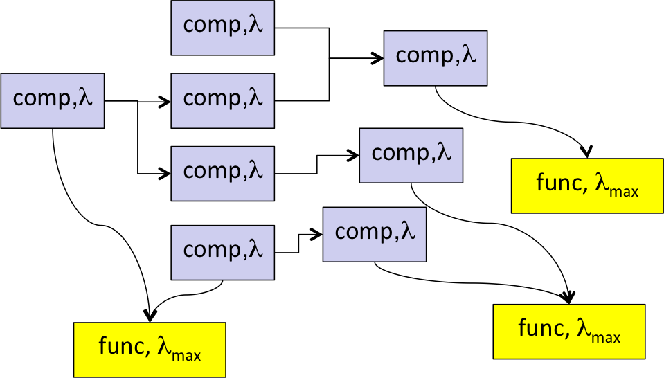
One of the core features to investigate in the context of RAMS analyses is the functional reliability of the system. Quantitatively represented by the failure rate lambda, it specifies the number of failures within a certain time period, e.g. “failures per million hours (fpmh)”.

Again as in post [001] we clearly have to distinguish between failure rates of system functions and of system components, as shown in the figure.

At the start of the design process what is given are probably upper limits of the failure rates of the functions – not the components (!) – of the designated system. These individual maximal values for lambda might be defined by the customer, by specification, by design rules, by standards (i.e. IEC 61508, ISO 26262, MIL882D etc) or otherwise. When developping a flexible block-library we need to represent this given parameter lambda_max by a value slot on function level.

On the other hand what has to be determined is each functions actual failure rate, say lambda_act. It depends mainly on 2 factors:

1. the failure rate lambda of each directly or indirectly required component, i.e. its quality
2. the system topology, how the components are connected and interact, i.e. the design architecture.

Concerning components quality, we simply provide a value slot on component level to represent the individual lambda. In the easiest case it will be just a fixed parameter for lambda. More ambitious approaches, like dependencies of the component’s failure rate on other environmental usage parameters, can be considered. In industrial practice also the “mean time between failures (mtbf)” is frequently used, which – under common conditions – is the inverse of the failure rate lambda.

Concerning system topology,. we need an arithmetic to consider the topology when determining the actual function failure rates. This is basically not too complicated, if we look at the system on a smaller, local or component scale instead trying to derive the calculation on global level. Assuming independence of the suppliers of a component, it follows simple rules, very similar to those applied in classical Fault Tree Analysis FTA:

1. Add up the probabilities of the individual failures, if each of them separately might “kill” the output. Example: The probability that an individual component fails to deliver its output service, is the sum of its own failure rate and the probability that its immediate supply fails.
2. Multiply the probabilities of the individual failures, if only the combination will “kill” the output. Example: The probability that the redundant supply of a component fails, is the product of the failure rates of the individual supplies.

Applying these rules recursively from the function viewpoint dependent on the individual redundancy situation at each component and its inputs, up to the first elements in the supplier-consumer-path, is a major step to modularize the failure rate computation of each function.

How closely related Fault Tree Analysis FTA and Root Cause Analysis are will be shown in post [004].