dependability.info

In this post we’re going to amend the existing library blocks by the quantities and arithmetics introduced in post [006] and see how this can facilitate the computation of the availability of a system.

What we need in the first step are the required variable and parameter slots, assigned to each individual item. For the time being we assume that the Mean Time To Repair MTTR is given as a known parameter for each item with the default unit of hours.

In the Modelica modeling language, parameters are quantities whose value has to be assigned prior to a simulation run, i.e. they will not be calculated. In that aspect the parameter type differs from normal variables. We plan to consider also other ways to determine and represent the MTTR and will describe this in future posts.

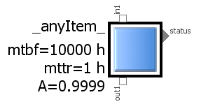
Since the Mean Time Between Failures MTBF has been introduced in a similar parametric way in the default item, the local availability A of this particular item may immediately be calculated according to the arithmetics in post [006]. So if the pre-assigned parameter values of MTBF is 10000 hours and the Mean Time To Repair is 1 hour, this results in a local item availability of 0.9999 or 99.99%. In case we want to achiev 99.999% i.e. five nines, we would have to modify e.g. MTTR to 0.1 hour – i.e. speed up the repair action – or increase MTBF to 100000 hours – i.e. get higher-quality parts. Since such modifications can be done interactively “on the fly”, this might help the system engineer to specify the quality requirements.

We may specify in the item graphics, that these parameter values shall be displayed besides the visual icon, along with the individual name (see intro figure).

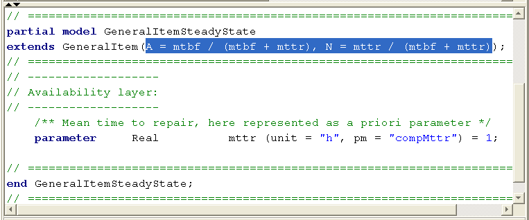
As the modeling approach follows an object-oriented concept, all item models are derived from one general item class and we need to do these declarations only at a single spot in the library. The next figure shows how this new functionality can be implemented very quickly in a few lines of code in the internal modeling language. Its only a reference to the GeneralItem master model, the equations for A and N and the declaration of the mttr parameter in a one-liner:

Before we proceed, it’s important to understand what we really have achieved now. We have just added the parameter MTTR to the master item description in the library. Such an item might represent various things like

• a certain technical hardware unit within a machine,
• a process step within a bigger procedure,
• an adminstrative item within an organisation
• or any other kind of element in a bigger context.

Together with the already existing parameter MTBF this allowed us to compute the also newly introduced availability quantity A. However, this item availability value is rather a theoretical value, describing a statistical value of this “box” in a standalone view, assuming that it is properly supplied.

In a real system, such an item almost never exists isolated. Instead, it will be connected to and interacting with its neighbors in a more or less complex environment. So in order to compute the actual service availability at the output of this box, we have to consider also the individual supply situation at its input. This will be the topic of post [008], then allowing us to efficiently compute the service availability of the power supply system from post [005]. And the good message is: this is possible without having to touch the overall system model!

Thanks for sharing this article!